Learn and Install Jupyter Notebook
Jupyter Notebook

This new tool is called Jupyter Notebook (or just Jupyter). Jupyter Notebook is much more complex than the code editor we've been working with. Using Jupyter, we can:
Type and execute code.
Add accompanying text to our code.
Add visualizations.
Source: jupyter.org
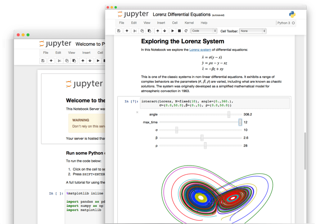
This combination of code, narrative text, and visualizations is a key element in almost any data science workflow. Jupyter makes it easy to combine these three elements, and this is what makes it a must-have tool for any data scientist. Jupyter is currently being used at multiple high-profile companies:
Source: jupyter.org

Jupyter Notebook is a web application, which means it can run in a browser. We'll use Jupyter Notebook constantly throughout our courses to work on portfolio projects. The big advantage of using Jupyter is that it allows you to easily share your projects with other people (employers included).
For instance, right after this mission, we'll use Jupyter to work on a guided project about Android and iOS mobile apps, and you'll be able to share a notebook like this (a notebook is a file created using Jupyter Notebook). We'll start learning how to use Jupyter Notebook in the next screen.
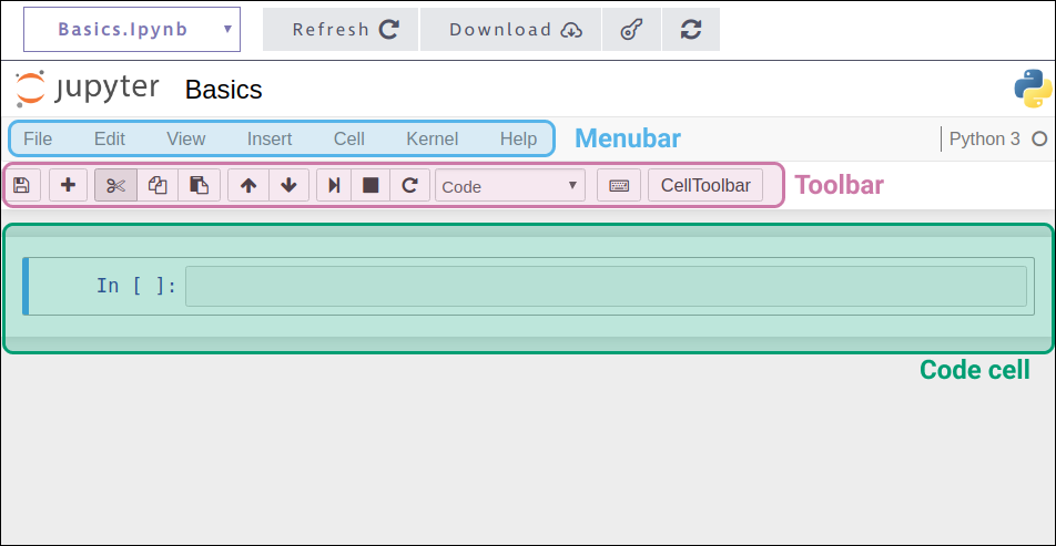
The Jupyter interface on the right of the screen has a few sections, including:
A menu bar
A toolbar
A code cell
To type and run code, we need to:
Click on the code cell.
Type the code we want to run.
Click the run cell, select below button on the toolbar.

Notice that after the code print('test code') finished running:
The string
'test code'was printed right below the code cell.A new code cell was inserted below the code cell we ran the code from.
We click on this second code cell and start writing more code. Then we click the run cell, select below button, which initiates the execution of the code and insert a new code cell below.

To edit any of the code we wrote, we need to click on a code cell and start editing. If we edit code in two cells or more, and then we want to run all the cells at once, we need to access the Cell menu on the menu bar, and then click on Run all. Below, we edit the code we ran above and then click Run all to run both cells in one go.

Now let's practice running code in Jupyter Notebook.
In the previous screen, we used the run cell, select below button to run code. It's more convenient, however, to use a keyboard shortcut to run code. The keyboard shortcut equivalent to the run cell, select below action is Shift + Enter.

The run cell, select below action runs code, but also inserts a new code cell below the cell we're executing the action from. Most of the time, we'll just want to run our code without inserting a new cell below. To do that, we can use the Ctrl + Enter shortcut, which doesn't insert any new cell.

Note that the run cell, select below action will insert a new cell only if there's no existing cell below the code cell we're executing this action from. If there's already a cell, then the run cell, select below action will just select that cell (hence the name run cell, select below), and won't insert any new cell.

We'll often want to insert a new cell even if there's already an existing cell below. To do that, we can use the run cell, insert below action, which always inserts a new cell below. This action can be done using Alt + Enter, or by clicking Run Cells and Insert Below in the Cell menu.
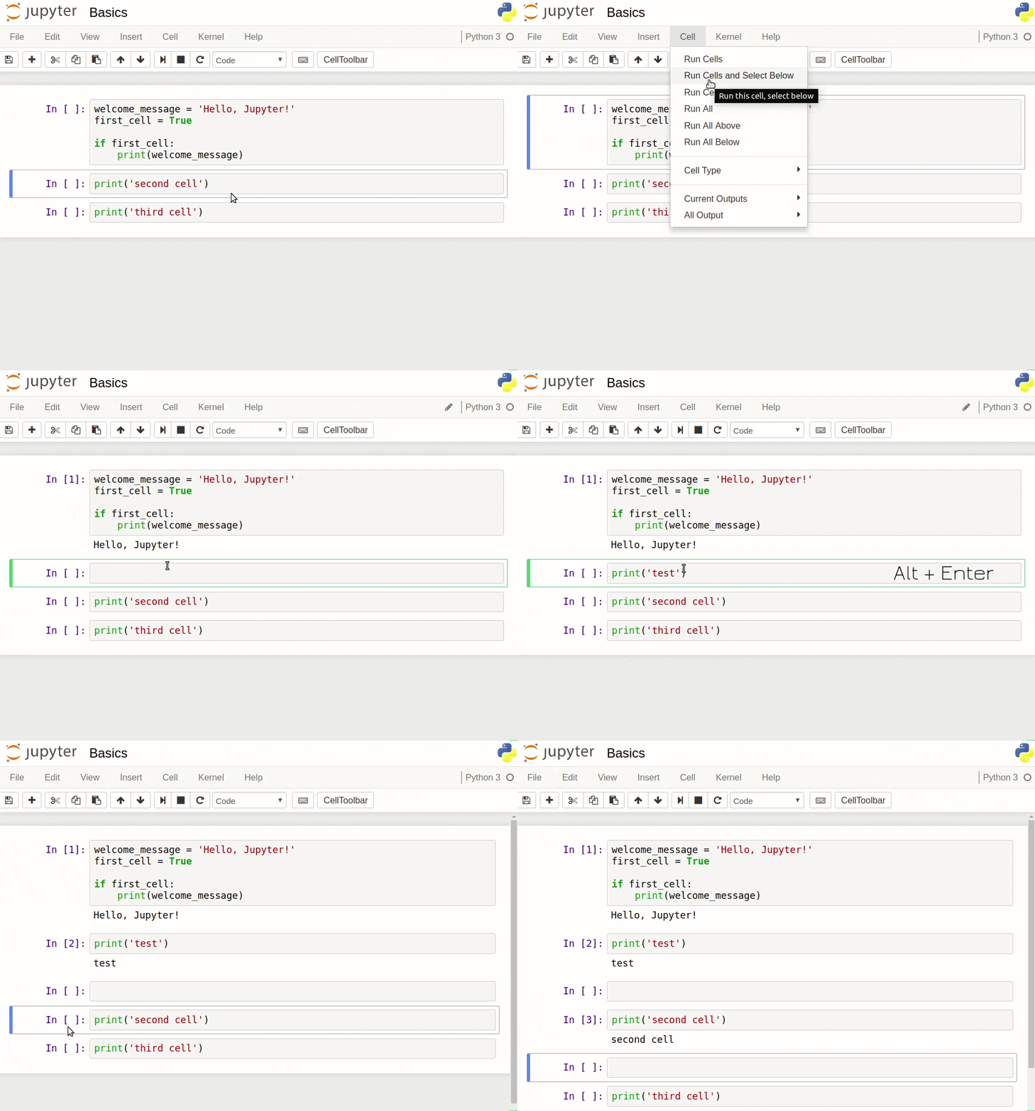
Let's now do a few exercises to practice the three keyboard shortcuts we discussed above:
Shift + Enter: run cell, select below
Ctrl + Enter: run selected cell
Alt + Enter: run cell, insert below
Instructions
In the first code cell, add
print('First cell'). Run all the code using the keyboard shortcut corresponding to the run cell, select below action.In the second code cell, add
print('Third cell'). Run all the code using the keyboard shortcut corresponding to the run selected cell action. Make sure that no new code cell is created below.Using only the keyboard, use the action run cell, insert below to insert a new cell between the current two cells. To do that:
Select the first cell using your mouse.
Run the first code cell using the keyboard shortcut corresponding to the run cell, insert below action.
Once the new code cell is created, type
print('Second cell')inside. Run the code, and make sure no new code cell is inserted below.
When we type code, Jupyter is in edit mode — a small pencil icon appears to the right of the menu bar when edit mode is active. If we press Esc or click outside the cell when Jupyter is in edit mode, Jupyter enters command mode — the pencil icon disappears when command mode is active.

It's useful to know the distinction between edit and command mode; each mode has specific keyboard shortcuts. If we go to the Help menu and click Keyboard Shortcuts, we can see the shortcuts specific to each mode.

Some of the most useful keyboard shortcuts we can use in command mode are:
Ctrl + Enter: run selected cell
Shift + Enter: run cell, select below
Alt + Enter: run cell, insert below
Up: select cell above
Down: select cell below
Enter: enter edit mode
A: insert cell above
B: insert cell below
D, D (press D twice): delete selected cell
Z: undo cell deletion
S: save and checkpoint
Y: convert to code cell
M: convert to Markdown cell (we'll talk about Markdown cells later in this mission)
Some of the most useful keyboard shortcuts we can use in edit mode are:
Ctrl + Enter: run selected cell
Shift + Enter: run cell, select below
Alt + Enter: run cell, insert below
Up: move cursor up
Down: move cursor down
Esc: enter command mode
Ctrl + A: select all
Ctrl + Z: undo
Ctrl + Y: redo
Ctrl + S: save and checkpoint
Tab: indent or code completion
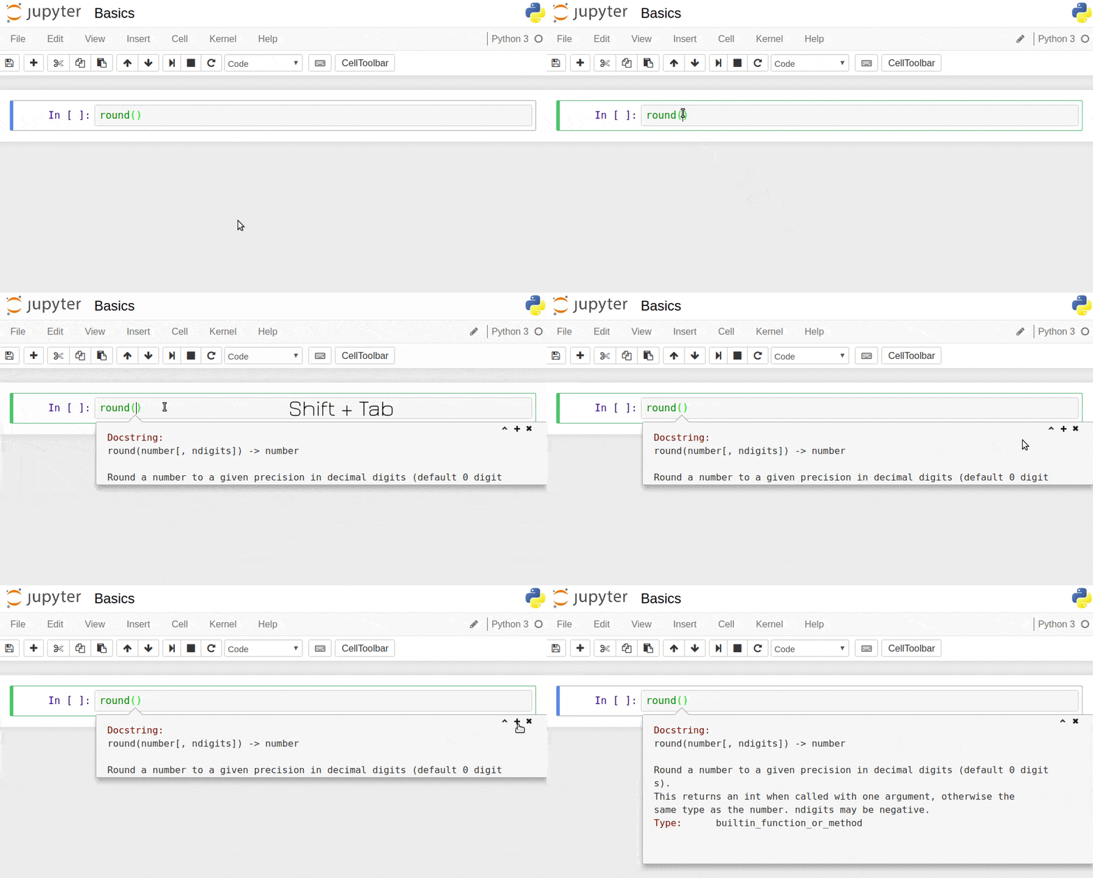
Shift + Tab: tooltip (for instance, if you press Shift + Tab while the cursor is within the parentheses of a built-in function, a tooltip with documentation will pop up)
A tooltip with documentation.
Note that some keyboard shortcuts are slightly different for MacBooks. If you have a MacBook, access the Help menu, and then click Keyboard Shortcuts to see all the keyboard shortcuts. Now, let's practice some of these keyboard shortcuts.
Instructions
Enter command mode by clicking the Jupyter interface somewhere outside the code cells, menu bar, and toolbar.
Select the second code cell using the Up and Down keys. This should be the cell containing only the code
print('Second cell').Delete this second code cell by pressing D twice: D, D.
Select the second code cell (which before deletion was the third code cell) using the keyboard and enter edit mode by pressing Enter.
Once in edit mode, use only your keyboard to change the code
print('Third cell')toprint('Second cell'). You can move the cursor using Up, Down, Left, and Right.Run the code in this second cell without creating any new cell below.
Enter command mode, select the second cell. Create a new cell below it by pressing B.
Enter edit mode in this new third cell, type the code
print('A true third cell'). Run the code cell while simultaneously creating a new cell below it.
Download this Jupyter Notebook for Follow above Instruction on this bellow notebook.
A variable or a function defined in a particular code cell becomes available in every other code cell. Below, we see that:
The
add_value()function is called in the second cell, although we defined it in the first cell.The variable
valis used in the second cell, although we defined it in the first cell.The variable
resultis used in the third cell, although we defined it in the second cell.

After we run code, the computer remembers what value is assigned to which variable, what function does what, etc. The sum of all this information that the computer remembers about our program is often called state or program state.
In our code example above, the state of our program is pretty complex and it includes information about:
The function
add_value()The variables
valandresultThe built-in functions, etc.
All the code cells of a Jupyter notebook share the same state. In our code example above, add_value(), val, and result are available across different cells because these different cells share the same state.
Now, let's get a better sense of how state is shared across different cells by doing a few exercises. We'll resume the discussion about state in the next screen.Instructions
Delete all the cells you created so far by pressing D, D.
In the first code cell:
Write a function named
welcome()that takes as input a parameter nameda_stringand prints the concatenated string'Welcome to ' + a_string + '!'. The function doesn't return anything, it just prints the string.Assign the string
'Dataquest'to a variable nameddq.Assign the string
'Jupyter Notebook'to a variable namedjn.Assign the string
'Python'to a variable namedpy.
Run the code in this first cell. Insert a new cell below.
In this newly created code cell, use the
welcome()function on the variablesdq,jn, andpy.
When we work in Jupyter, we usually run code cells in order (from top to bottom), and this helps us keep a clear mental picture of our program's state.
However, sometimes we may want to go back and add some changes to certain code cells, and then run the code in those specific cells again. Jupyter is flexible enough to allow us to do that, but this is a double-edged sword — it can easily make us lose track of our program's state.
In the code example below, we modified a bit of the program we wrote on the previous screen, and:
Edited
add_value()to returnx + 30instead ofx + 5.Changed the value we assign to
valfrom15to20.Ran the first code cell.
Left the other code cells untouched (we didn't run them again).

The modified code may be extremely confusing if we see it for the first time or forgot the small changes we made (this is common when writing large programs). By reading the first two cells of the modified code, you can think about the program's state and deduce that result should be 50. However, in the third cell, we see that result is actually 20.
This most likely happened because there's something in the program's state we're not aware of — the program has some hidden state. To find out what's really happening, we can start by checking the order of code execution. The numbers in In [number]:, which we can see on left of each code cell, provide us with the order of execution.
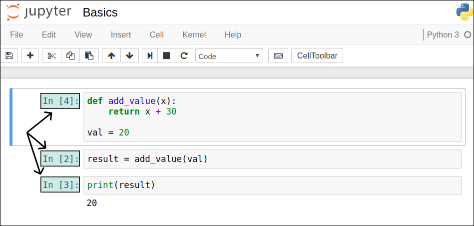
Above, we see the first cell has In [4]: on its left, which tells us that it was the fourth cell to run. The second cell has In [2]:, so it was the second cell to run, and the third cell has In [3]:, so it was the third cell to run. In [1]: is missing, which tells us that either:
One of the existing code cells has run again (and was possibly edited); or
A code cell ran and was then deleted.
To find out exactly what happened, we can run the special command %history -p, which tells what code ran in what order:

The >>> symbol we see in the output of %history -p corresponds to an individual code cell. We can see that:
In the first code cell that was run, the
returnstatement wasreturn x + 5(instead ofreturn x + 30) andvalwas15(instead of20).In the second cell, we assigned the output of
add_value(val)toresult.In the third cell, we printed
result.In the fourth cell, we ran
add_value()with a modifiedreturnstatement (return x + 30instead ofreturn x + 5). We also ranval = 20(as opposed toval = 15).In the fifth cell, we ran
%history -p.
The history of code execution we see above tells us a few things:
The
add_value()function and thevalvariable were modified.result = add_value(val)andprint(result)were not run again afteradd_value()andvalwere modified.
To fix the issue, we can run the second and the third cell again, and result will become 50, just as expected:

In practice, the solution is not always as obvious as above. The best thing to do is to restart the state and run again all the code cells in order from top to bottom. We can easily do that by clicking Restart & Run All in the Kernel menu.

Now let's practice to get a better grasp of hidden states.Instructions
Run the
%history -pcommand to get an understanding of the current state of your program.The output of
%history -pshould be pretty verbose since we ran quite a lot of code so far — you should also see that it's not very easy to understand the state of the program at this point.
Restart the state of your program and clear the output of every cell by clicking the Restart & Clear Output action from the Kernel menu.
In a separate cell, run the
%history -pcommand again to confirm that no code has been run (except for%history -p).Run the code we wrote in the previous exercise again.
Modify the first cell (the one where you defined only the function
welcome()and the variablesdq,jn, andpy):The function should not print the string
'Welcome to ' + a_string + '!'anymore. Instead, the string'Welcome to ' + a_string + '!'is saved to a variable and the variable is returned (using areturnstatement).Delete the line of code where you assigned the string
'Python'to thepyvariable.
Run the modified code, and then try to think about the state of the program just by using the code and the output you see.
You should notice that the state you deduced is contradictory to the output printed in the second cell — for instance,
welcome(dq)is not supposed to print anything (because we didn't useprint()this time), andwelcome(py)should raise an error becausepyis not defined anymore.
Pretend you don't know what happened exactly and run the
%history -pcommand again to find out.Fix the issue either by running the second code cell again or by clicking Restart & Run All in the Kernel menu.
One of the most useful features of Jupyter is that it allows us to accompany our code with text.

Accompanying code with text is useful because it allows us to document or explain our code — similar to how we explained our code in the example above. More relevant to the data analysis workflow, however, text enables us to detail our analysis by providing thorough explanations of the steps we take to analyze data. In the next guided project, for instance, we'll use text extensively to explain the steps of our analysis.
In the example below, we show how to add text to explain our code. To do that, we:
Create a new code cell above our current code cell.
Convert the new code cell to a Markdown cell by clicking
Markdownon the dropdown menu found on the toolbar.Add a snippet of text to explain the behavior of our code. We type "In the code below, we will:" and then we paste the rest of the text.
Click the run cell, select below button on the toolbar to run the cell (we can also use the shortcuts Shift + Enter, Alt + Enter, or Ctrl + Enter).

The kind of cell we use to add text is called "Markdown" because it supports Markdown syntax. Markdown syntax allows us to use keyboard symbols to format our text such that we can:
Add italics and bolds.
Add headers (titles) of various sizes.
Add hyperlinks and images.
For instance, below we double-click the Markdown cell to enter edit mode, and then we edit the text using Markdown syntax:
We add the title "My Data Science Project" using the syntax
# My Data Science Project— we added the#character in front ofMy Data Science Project.We highlight all the code elements by surrounding them with backticks.

You can find a useful cheat sheet on Markdown syntax at this link. It should take you less than two minutes to read it, and you will learn what syntax to use to:
Add italics and bolds.
Add headers (titles) of various sizes.
Add hyperlinks and images.
Add block quotes.
Add lists.
Add horizontal lines (useful to delimit the sections of a big project).
Add inline code.
Add code blocks.
Now let's practice adding text and using the Markdown syntax. Note that you'll need to access and read the cheat sheet above to solve the exercise.Instructions
In a code cell, open the
AppleStore.csvdata set. Read it in as a list of lists, and display the first few rows.If you run into an error named
UnicodeDecodeError, addencoding="utf8"to theopen()function (for instance, useopen('AppleStore.csv', encoding='utf8')).
Create a Markdown cell above the code cell you used to open the data set and explain the steps you took to open the data set.
Below the code cell, add another Markdown cell, where you give some information about the data set you just opened. Assume you're writing for someone who doesn't know anything about the data set. Mention:
What the data set is about
The source of the data set
Where the data set can be downloaded from and where the documentation can be found — add a hyperlink to the documentation
Finally, use Markdown syntax to create a table like the one below to explain what each column in the data set is about. Use this resource to quickly learn the syntax for adding a table. You can find what each column describes by reading the documentation of the data set.
Column name
Description
"id"
App ID
"track_name"
App Name
"size_bytes"
Size (in Bytes)
.....
.....
At Dataquest, we strongly advocate project-based learning. For this reason, we created a large number of guided projects. As you work on guided projects, you can either:
Work directly in our interface using Jupyter Notebook; or
Work locally by installing Jupyter Notebook on your own computer.
There's more than one way to install Jupyter on your computer. If you're a more experienced Python user, you may want to install Jupyter using pip (Python's package manager). Older versions of pip may have trouble with some dependencies, so make sure you first run pip3 install --upgrade pip in the command line. Then, you can install Jupyter by running pip3 install jupyter.
If you're new to Python, we strongly recommend installing the Anaconda distribution, which will install both Python and Jupyter on your computer. You can download the Anaconda distribution from here.
Before you start downloading, make sure you:
Select the right operating system — Windows, macOS, or Linux.
Download the Python 3 version.

Note that Python 2 is an older version of Python; it will stop being maintained after 2020. At Dataquest, we teach Python 3, which is what most people in the Python community use.
After you finished downloading, install Anaconda using one of these guides:
After you finished installing Anaconda, open the Anaconda Navigator by following the instructions here. Navigator's Home screen displays several applications you can choose from — one of them is Jupyter Notebook. Click on the Launch button to launch Jupyter.

Jupyter Notebook is a web application, and a new web page will pop up in your browser after you click the Launch button. In the next screen, we'll discuss how to open a notebook file and start coding.
As soon as you launch Jupyter, a new web page pops up in the browser. Jupyter is a web application, which means it runs in the browser. A new server is created at localhost:8888, the URL you see in the browser.

Access to your notebook server is restricted via a token-based authentication that Jupyter runs by default. You don't need to worry that random people on the Internet can access the server and run arbitrary code. You can read more about the security in a Jupyter notebook server here, and you can find more technical details about the kind of server Jupyter runs here.
To create a new notebook file, we need to click on the New dropdown menu and then select Python3. This will automatically create and open a new notebook file which we can use to run Python 3 code. After the notebook file is open, you should see the same Jupyter interface that you've been seeing on the Dataquest website.

When you want to stop working, you'll need to save your file, then click Close and Halt from the File menu, which will close the current notebook file.

In previous missions, we opened the AppleStore.csv file several times. But now that we've installed Jupyter locally, we may want to try to open the file AppleStore.csv on our own computer.
Let's say we downloaded the AppleStore.csv file and saved it into a directory named my_datasets — a directory which exists at the location /home/alex/my_datasets.

Now that we have the CSV file on our computer, we should be able to open it using the code open('AppleStore.csv'). Below, we:
Create a new notebook file.
Try to open the
AppleStore.csvfile using the codeopen('AppleStore.csv').

We see that we got a FileNotFoundError, which tells us there's no such file or directory on our computer named AppleStore.csv. However, we know for sure there is a CSV file named AppleStore.csv located at /home/alex/my_datasets.
To debug the code, we'll need to specify the exact path (location) of the file, which is /home/alex/my_datasets. We'll also need to add the file name, so we'll add /AppleStore.csv at the end of that path, ending up with /home/alex/my_datasets/AppleStore.csv.
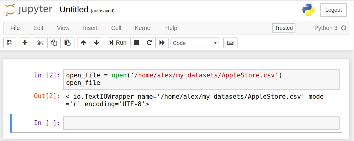
When we use open('AppleStore.csv') (without specifying the full path), the computer looks for the AppleStore.csv file only inside the directory where the notebook from which we run code is located. For example, above we ran open('AppleStore.csv') from the Jupyter notebook we had created initially, which was named Untitled.ipynb by default and saved at /home/alex.
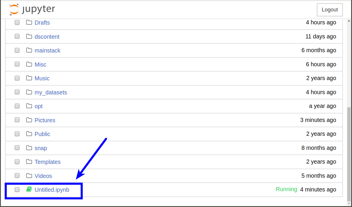
If we run open('AppleStore.csv') from the Untitled.ipynb notebook, the computer only searches inside the /home/alex directory (without opening any subdirectory that exists at /home/alex). Since the AppleStore.csv file is located at /home/alex/my_datasets, and the computer only searches within /home/alex (without looking into subdirectories), the computer is not able to locate the file and throws a FileNotFoundError.
Now that we know the computer only searches within the directory of the notebook file, we can also debug our initial code by bringing the notebook file and the data set in the same directory. There are at least two ways we can do that:
We can create a new notebook at
/home/alex/my_datasets(whereAppleStore.csvis located) and runopen('AppleStore.csv')from there.We can copy the
AppleStore.csvfile to/home/alex.
To create a new notebook at /home/alex/my_datasets, we need to access the my_datasets directory from the Jupyter interface, and then we can create the notebook.

Copying AppleStore.csv to /home/alex is simply a matter of copy-paste. Once the data set is pasted at /home/alex, we can directly use open('AppleStore.csv').

The full path of a file (like /home/alex/my_datasets/AppleStore.csv) is often known as the absolute path. When we used open('/home/alex/my_datasets/AppleStore.csv'), we specified the absolute path.
When we used open('AppleStore.csv'), we specified the relative path of the file. A relative path is always relative with respect to a certain directory — in our last example above, the relative path was relative to the directory of the notebook file, which was /home/alex.
Jupyter Notebook was the focus of this mission, and we learned:
How to run code using Jupyter
How to add text using Jupyter
How to install Jupyter locally
We've made great progress in this course and learned about:
The basics of programming in Python (arithmetical operations, variables, common data types, etc.)
List and for loops
Conditional statements
Dictionaries and frequency tables
Functions
Jupyter Notebook
Next, we'll work together on a guided project to apply what we've learned.
Review
Syntax
MARKDOWN SYNTAX
Adding italics and bold:
*Italics* **Bold**Adding headers (titles) of various sizes:
# header one ## header twoAdding hyperlinks and images:
[Link](http://a.com)Adding block quotes:
> BlockquoteAdding lists:
* * *Adding horizontal lines:
‐‐‐Adding inline code:
`Inline code with backticks`Adding code blocks
``` code ```
JUPYTER NOTEBOOK SPECIAL COMMAND
Displaying the code execution history:
%history -p
Concepts
Jupyter Notebook is much more complex than a code editor. Jupyter allows us to:
Type and execute code.
Add accompanying text to our code (including math equations).
Add visualizations.
Jupyter can run in a browser and is often used to create compelling data science projects that can be easily shared with other people.
A notebook is a file created using Jupyter notebooks. Notebooks can easily be shared and distributed so people can view your work.
Types of modes in Jupyter:
Jupyter is in edit mode whenever we type in a cell — a small pencil icon appears to the right of the menu bar.
Jupyter is in command mode whenever we press Esc or whenever we click outside of the cell — the pencil to the right of the menu bar disappears.
State refers to what a computer remembers about a program.
We can convert a code cell to a Markdown cell to add text to explain our code. Markdown syntax allows us to use keyboard symbols to format our text.
Installing the Anaconda distribution will install both Python and Jupyter on your computer.
Keyboard Shortcuts
Some of the most useful keyboard shortcuts we can use in command mode are:
Ctrl + Enter: run selected cell
Shift + Enter: run cell, select below
Alt + Enter: run cell, insert below
Up: select cell above
Down: select cell below
Enter: enter edit mode
A: insert cell above
B: insert cell below
D, D (press D twice): delete selected cell
Z: undo cell deletion
S: save and checkpoint
Y: convert to code cell
M: convert to Markdown cell
Some of the most useful keyboard shortcuts we can use in edit mode are:
Ctrl + Enter: run selected cell
Shift + Enter: run cell, select below
Alt + Enter: run cell, insert below
Up: move cursor up
Down: move cursor down
Esc: enter command mode
Ctrl + A: select all
Ctrl + Z: undo
Ctrl + Y: redo
Ctrl + S: save and checkpoint
Tab : indent or code completion
Shift + Tab: tooltip
Resources
Jupyter Notebook tutorial
Jupyter Notebook tips and tricks
Markdown syntax
Installing Anaconda
Last updated